Page 65 - RSE - Results of the Apollon Project
P. 65
67 Results of the APOLLON project and Concentrating Photovoltaic perspective
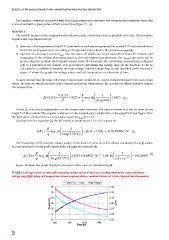
From the data of Figure 70, for each current value, a linear regression of the junction voltage against the
temperature value can be calculated. (see Figure 71 a))
76
y = -0.1028x + 77.33
-0,090
74
VOLTAGE TEMPERATURE
1,20
1,00
0,80
0,40
0,20
-0,0950,00
0,60
72
y = -0.1143x + 74.187
-0,100
COEFFCIENT (V/°C)
0.02
-0,105
70
V (V)
0.21
-0,110
68
-0,115
0.82
-0,120
y = -0.1334x + 68.966
66
-0,125
64
-0,130
-0,135
62
-0,140
25 27 29 31 33 35 37 39 41
I(A)
T (°C)
b)
a)
Figure 71 a) Voltage–temperature linear regression at different current values (A) depicted on the right side of the
graph, b) Voltage – temperature coefficient in function of the current.
Results of the APolloN PRoject ANd coNceNtRAtiNg PhotovoltAic PeRsPective
The angular coefficient associated to each linear regression represents the temperature coefficient value that is
associated to a given value of dark current (see Figure 71 b)).
The angular coeffcient associated with each linear regression represents the temperature coeffcient value that
is associated with a given value of dark current (see Figure 71 - b).
Method B
The module under test is equipped with a thermocouple, attached as close as possible to the cell.
METHOD B The procedure requires two experimental steps:
The module being tested is equipped with a thermocouple, attached as close as possible to the cell. The procedure
1) detection of an experimental dark I-V curve with an ambient temperature Tin around 25°C
requires two experimental steps: and identification of the electrical parameters, according to the procedure described in
the previous paragraph.
1) detection of an experimental dark I-V curve with an ambient temperature Tin around 25°C and identifcation
2) Injection a constant current I therm into the solar cell which, for Joule effect heats the module and
of the electrical parameters, according to the procedure described in the previous paragraph;
acquiring the voltage decreasing trend as the cell temperature increases. The I therm value hasn’t to
2) injection of a constant current I into the solar cell which, due to the Joule effect heats the module, and
therm be greater than the module short circuit current value. To determine the cell voltage temperature
acquisition of the voltage decreasing trend as the cell temperature increases. The I therm value must not be
coefficient β C(I) in function of the current, it is necessary to determine the voltage drop on the
greater than the module short circuit current value. To determine the cell voltage temperature coeffcient
junction. It can be calculated as a difference between the total voltage and the voltage drop on
(I) as a function of the current, it is necessary to determine the voltage drop on the junction. It can be
C the identified series resistance. Figure 72 shows the graphs of voltage values and cell
calculated as a difference between the total voltage and the voltage drop on the identifed series resistance.
temperature in function of the time.
Figure 72 shows the graphs for voltage values and cell temperature as a function of time.
It can be shown that the solar cell voltage temperature coefficient, βc, can be considered equal to the sum of two
It can be shown that the solar cell voltage temperature coeffcient, , can be considered equal to the sum of two
c
terms: the first one which depends on the current and on the temperature, the second one, which depends only on
terms: the frst one which depends on the current and on the temperature, the second one, which depends only on
the temperature: the temperature:
V (I ,T ) K I
β C (I ,T ) = + b (T ) = neq ⋅ ln + b (T ) (2),
(2)
T q Ioeq (Tin )
In reality, β c it is almost independent on the temperature, therefore, the determination of β can be done at any
single T of the module. The angular coefficient of the interpolating straight-line of the graph V-T (see Figure 73) is the
In fact, it is almost independent on the temperature, therefore, the determination of can be done at any
68 Results of the APOLLON project and Concentrating Photovoltaic perspective
c
68 Results of the APOLLON project and Concentrating Photovoltaic perspective
β C(I) value calculated for a current value equal to I therm (= 1.5 A).
single T of the module. The angular coeffcient of the interpolating straight-line of the graph V-T (see Figure 73) is
the (I) value calculated for a current value equal to I (= 1.5 A).
C therm
Starting from the equation (2), the b(T) value at temperature T= 27.2°C is given by:
Starting from the equation (2), the b(T) value at temperature T= 27.2°C is given by:
K I
)
b( T =) neq ⋅ln K I − β C I ( = 5.1 A = − 014909.0 V ° / C (3)
)
neq ⋅ln
° 2. 7(
q b( T =) q Ioeq 2 C) ° 2. 7( C) − β C ( I = 5.1 A = − 014909.0 V ° / C (3) (3)
Ioeq 2
The knowledge of b(T) and the voltage values of the dark I-V curve at 27.2°C, allows calculating the βC(I) values in
The knowledge of b(T) and the voltage values of the dark I-V curve at 27.2°C, allows calculating the βC(I) values in
The knowledge of b(T) and the voltage values of the dark I-V curve at 27.2°C, allows calculating the C (I) values
correspondence of any dark current value by using the formula (4):
correspondence of any dark current value by using the formula (4):
in correspondence of any dark current value by using the formula (4):
K I − 5 I (4)
β C (I ) = neq ⋅ ln K + I (Tb ) = 6532.8 ⋅ 10 83 ⋅ 8. ⋅ − ln 5 − I 014909. 0 (4)
ln
⋅ −
q β C (I ) = q neq 2 ⋅ ln °C ) 2 2. 7( Ioeq °C ) + b (T ) = . 8 6532⋅ 10 33 83 ⋅ 1. 8. ⋅ 10 14 1. − 14 − . 0 014909 (4)
2. 7( Ioeq
33 ⋅ 10
Figure 74 shows the graph of C (I) as a function of the current calculated by (4).
Figure 74 shows the graph of βC(I) in function of the current calculated by (4).
Figure 74 shows the graph of βC(I) in function of the current calculated by (4).
FiguRE 72. Voltage values of solar cell (magenta), voltage values of the solar cell depurated of the series resistance
voltage drop (light blue), cell temperature values acquired while a constant current of 1.5A is injected into the receiver
Tcell (°C) Vcell Vcell -Rseq*I
Tcell (°C) Vcell Vcell -Rseq*I
55 3.15
55 3.15
50 3.13
50 3.13
45 45 3.11 3.11
Tcell (° C) 40 Tcell (° C) 40 3.09 V (V) 3.09 V (V)
3.07
35
30 35 3.05 3.07
30 3.05
25 3.03
25 3.03
200 700 1200 1700
200 Time (s) 1200 1700
700
Time (s)
Figure 72. Voltage values of solar cell (magenta), voltage values of the solar cell depurated from the series resistance
Figure 72. Voltage values of solar cell (magenta), voltage values of the solar cell depurated from the series resistance
voltage drop (light blue), cell temperature values acquired while a constant current of 1.5A is injected into the
64 voltage drop (light blue), cell temperature values acquired while a constant current of 1.5A is injected into the
receiver.
receiver.
3.15
3.15
3.13
3.13 y = -0.004344x + 3.255824
y = -0.004344x + 3.255824
2
3.11 R = 0.999920
2
3.11 R = 0.999920
V (V) 3.09 V (V) 3.09
3.07
3.07
3.05
3.05
3.03
3.03
27 29 31 33 35 37 39 41 43 45 47 49 51 53
37
35
27 29 31 33 T (°C) 39 41 43 45 47 49 51 53
T (°C)
Figure 73. Graph of the solar cell voltage depurated from the series resistance in function of the temperature and for
Figure 73. Graph of the solar cell voltage depurated from the series resistance in function of the temperature and for
I= Itherm= 1.5 A
I= Itherm= 1.5 A